Excel Macro to run trade report on DAS Trader Pro trade log

I have been mucking about with some programming lately and I only just realized that the work I had been doing to get my average price on trades so I can enter it into my trade log was easily automated. The below Excel (2010 is the version I use) macro has made my life a little easier so I am sharing it here. This can be used with the ‘trade’ output of DAS Trader Pro (which I am currently using with Centerpoint Securities) but with slight changes could be used on the output from Sterling Trader Pro or other trading platforms. There are easier ways to get the summaries, but I make sure to record trades I make in my trade log with details including my trade plan and post-trade evaluation — most of the time I’ll put together all the trades in each ticker to save time and because I’m trading the stock with one strategy. So for my purposes I like having the average price (including fees) shown neatly.

First, start with how the data should be formatted prior to the macro working. Go to “Trade” in DAS Trader Pro and then click “Trades”. Select the columns and copy and paste into an Excel worksheet named “scratchpad” (and make sure to paste into column B). Then hit Control + A to select the entire range of data and run the macro (I have it hotkeyed on my computer to Control+P). This will create a new worksheet, run a pivot table, copy the pivot table data, delete the pivot table worksheet, and paste the pivot table data and price per share in an easy to read format in another new worksheet.

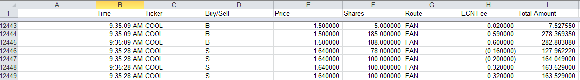
Here is how the data should be formatted in your trade report that you paste into Excel (you do not need a header row):

inputdata

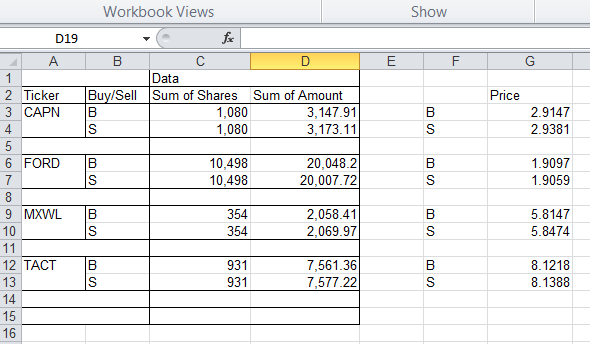
And below is how the data will be output:

macro_output

Obviously, you can use this same basic code framework to get lots of other data easily (such as ECN fees, etc). The one thing this code will not do is account for per-trade fees. I don’t have them at Centerpoint (clearing through ETC) so I didn’t program them. Also, make sure you enter your per-share commission into the code. Use this code at your own risk — I provide it without warranty or support.

Warning: if you are a programmer you will find my code ugly. You have been warned.

Below is the code:

Sub DAStraderAvgPrices()

‘ DAStraderAvgPrices Macro
‘ For this to work you need to copy pasta the following columns from DAS into the ‘sheet ‘scratchpad’
‘Time | Ticker | Buy/Sell | Price | Shares | Route | ECN Fees | Amount of trade
‘Those columns all must be there in that order or it will mess lots of things up.
‘The trades must be pasted into column B and then select all the trade info ‘(control+A)

Dim myRange As Range
Dim i As Long
Dim HeaderRange As Range
Dim HeaderPasteRange As Range
Dim TopLeft As Range
Dim objTable As PivotTable
Dim objField As PivotField
Dim rng As Range
Dim ws1 As Worksheet
Dim pt As PivotTable
Dim rngPT As Range
Dim rngPTa As Range
Dim rngCopy As Range
Dim rngCopy2 As Range
Dim lRowTop As Long
Dim lRowsPT As Long
Dim lRowPage As Long
Dim PivotTableSheet As String
Dim celltxt As String

‘this is my commission rate
commission = 0.0035

Set myRange = Selection

‘sort by column C then D (ticker then buy/sell)
myRange.Sort Key1:=Columns(3), Order1:=xlAscending, Key2:=Columns(4) _
, Order2:=xlAscending, Header:=xlGuess, OrderCustom:=1, MatchCase:= _
False, Orientation:=xlTopToBottom
‘the above works! Yay!

‘this section calculates the cost basis (including ECN fees and commissions) of each fill
For i = myRange.Rows.Count To 1 Step -1
Set BuySell = myRange.Cells(i, 3)
If BuySell.Value = “B” Then
myRange.Cells(i, 8) = (myRange.Cells(i, 4) + commission) * myRange.Cells(i, 5) + myRange.Cells(i, 7)
ElseIf BuySell.Value = “S” Then
myRange.Cells(i, 8) = (myRange.Cells(i, 4) – commission) * myRange.Cells(i, 5) – myRange.Cells(i, 7)
ElseIf BuySell.Value = “SS” Then
myRange.Cells(i, 8) = (myRange.Cells(i, 4) – commission) * myRange.Cells(i, 5) – myRange.Cells(i, 7)
End If
Next i

‘Here we append the header row to the data
myRange.Cells(0, 1) = “Time”
myRange.Cells(0, 2) = “Ticker”
myRange.Cells(0, 3) = “Buy/Sell”
myRange.Cells(0, 4) = “Price”
myRange.Cells(0, 5) = “Shares”
myRange.Cells(0, 6) = “Route”
myRange.Cells(0, 7) = “ECN Fee”
myRange.Cells(0, 8) = “Amount”

‘Pivot table time!

‘only uncomment the following two lines when testing on specific region
‘ActiveWorkbook.Sheets(“scratchpad”).Select
‘Range(“B4”).Select

ActiveWorkbook.Sheets(“scratchpad”).Select
myRange.Cells(0, 1).Select

Set objTable = ActiveSheet.PivotTableWizard

Set objField = objTable.PivotFields(“Ticker”)
objField.Orientation = xlRowField
objField.Position = 1

Set objField = objTable.PivotFields(“Buy/Sell”)
objField.Orientation = xlRowField
objField.Position = 2

Set objField = objTable.PivotFields(“Shares”)
objField.Orientation = xlDataField
objField.Position = 1
objField.Function = xlSum
objField.NumberFormat = “##,###”

Set objField = objTable.PivotFields(“Amount”)
objField.Orientation = xlDataField
objField.Position = 2
objField.Function = xlSum
objField.NumberFormat = “##,###.##”

‘Pivot tables with multiple data fields have hidden field “data” —
‘adding the below line makes it display correctly
objTable.AddFields Array(“Ticker”, “Buy/Sell”), “Data”

‘Copy the Pivot table and paste it into a new worksheet as values
On Error Resume Next
Set pt = ActiveCell.PivotTable
Set rngPTa = pt.PageRange
‘On Error GoTo errHandler

PivotTableSheet = ActiveSheet.Name

‘If pt Is Nothing Then
‘ MsgBox “Could not copy pivot table for active cell”
‘ GoTo exitHandler
‘Else
Set rngPT = pt.TableRange1
lRowTop = rngPT.Rows(1).row
lRowsPT = rngPT.Rows.Count
Set ws1 = Worksheets.Add
Set rngCopy = rngPT.Resize(lRowsPT – 1)
Set rngCopy2 = rngPT.Rows(lRowsPT)

rngCopy.Copy Destination:=ws1.Cells(lRowTop, 1)
rngCopy2.Copy Destination:=ws1.Cells(lRowTop + lRowsPT – 1, 1)
‘End If

If Not rngPTa Is Nothing Then
lRowPage = rngPTa.Rows(1).row
rngPTa.Copy Destination:=ws1.Cells(lRowPage, 1)
End If

ws.Columns.AutoFit

‘Stopping Application Alerts
Application.DisplayAlerts = False

‘delete pivot table sheet
Sheets(PivotTableSheet).Delete

‘Add in some formatting and get price per share for buys/sells

Columns(“C:C”).ColumnWidth = 13.71
Columns(“D:D”).ColumnWidth = 14.86
Range(“G2”).Select
ActiveCell.FormulaR1C1 = “Price”
Columns(“G:G”).Select
Selection.NumberFormat = “0.0000”
Selection.ColumnWidth = 11.43
Range(“F3”).Select
ActiveCell.FormulaR1C1 = “=IF(ISBLANK(RC[-4]),””””,RC[-4])”
Range(“F3”).Select
Selection.AutoFill Destination:=Range(“F3:F197”), Type:=xlFillDefault
Range(“F3:F197”).Select
Range(“G3”).Select
ActiveCell.FormulaR1C1 = _
“=IF(ISBLANK(RC[-3]),””””,IF(ISBLANK(RC[-5]),””””,RC[-3]/RC[-4]))”
Range(“G3”).Select
Selection.AutoFill Destination:=Range(“G3:G202”), Type:=xlFillDefault

‘Loop through table to clear all rows that contain “Total”
Last = Cells(Rows.Count, “D”).End(xlUp).row
For i = Last To 1 Step -1
celltxt = Cells(i, “A”).Text
If InStr(1, celltxt, “Total”) Then
Cells(i, “A”).EntireRow.ClearContents ‘ USE THIS TO CLEAR CONTENTS BUT NOT DELETE ROW
End If
Next i

ActiveSheet.UsedRange.Select

exitHandler:
Exit Sub
errHandler:
MsgBox “Could not copy pivot table for active cell”
Resume exitHandler
End Sub


Disclaimer: I have no position in any stocks mentioned as of this post being published but I may trade them in the future. I am a client of Centerpoint Securities (clearing through ETC). I have no relationship with any other parties mentioned above. This blog has a terms of use that is incorporated by reference into this post; you can find all my disclaimers and disclosures there as well.

We are all in this together … or not

Whenever you hear that phrase, “We’re all in this together,” be very, very cautious. That is what scammers will say to convince you to do stupid things with your money (like buying pumped stocks) and what both hucksters and even non-fraudulent trading gurus will say to try to get their hands on your money.

The simple truth of the matter is that everyone has different goals and priorities. The most important thing you can do is to make sure you are aware of how the priorities of those you deal with and listen to differ from your own. A stock promoter’s goal is simply to get you to buy stock — damn you and your kid’s college fund.  A trading guru who sells his services with an alert service or trading chatroom benefits the longer you subscribe. His financial interest is best served by selling something that you will continue to want or need for years and years. The guru’s monetary motivation will — ceteris paribus of course — cause him to charge as much as he can for as little as he can. He will sell you hard to get you to pay him more money.

Even saying that all traders care about is profits is wrong. Especially in the penny stock world there are many of us who are motivated by other things besides profits (of course we are all motivated to a large extent by profits). I remember getting a bunch of flak from commenters on this blog when I accused a certain pumper of violating securities laws (six months later the SEC sued him). People attacked me for potentially destroying profitable trading opportunities. But I along with most other bloggers don’t just do this for money.

At the end of the day, each of us is motivated by different things, some of which are obvious, some of which are not. Money is the most obvious, but most of have emotional motivations — we genuinely want to help those we come across. Some of us have other motives that drive us, more powerful motives. When the time comes, my motivations will be made clear. In the meantime, let us embrace the motto “All for one, one for all, and every man for himself!”


Disclaimer: No positions in any stocks mentioned. This blog has a terms of use that is incorporated by reference into this post; you can find all my disclaimers and disclosures there as well..

Deep Springs: A lesson in randomness

Longtime readers will know that I stress the importance of randomness in investing and trading. Any investing or trading strategy will produce a number of losers. Sometimes these losing trades or investments will cluster together purely by chance; it can be difficult to distinguish these chance losing streaks from a declining in a trading system’s performance.

Those without statistics training may find it difficult to think in probabilistic terms and and often do not realize how random the world truly is. Following is a real life example of randomness in action. Take two bright, motivated, and somewhat unusual young men, just five years apart in school, both living in the Chicago metropolitan area. One of them, named Michael, attends a pretty good suburban high school. The other, named Franklin, attends the state math and science magnet school. When it comes time, both apply to a number of colleges, including the most exclusive and unusual college in the country, Deep Springs.

The application process to get into Deep Springs is the most demanding application to any undergraduate institution in the country. After writing over 20 pages of essays each, submitting recommendations and standardized tests, both Michael and Franklin are given the chance to visit Deep Springs where they face a second screening, intended to winnow the applicants further (this is early in 1999 for Michael and 1995 for Franklin). One is rejected, the other accepted. Here their paths diverge.

Franklin attends Deep Springs for two years and then transfers to Harvard. He graduates with high honors, marries, and then works for three years in a psychology research lab at Brandeis University. He then applies and is accepted to enter the Psychology PhD program at Washington University in St. Louis, under renowned researched Henry L. Roediger III.

Five years after Franklin is accepted by Deep Springs, Michael is rejected by Deep Springs and instead he begins college at Grinnell College in Iowa, a well-respected liberal arts college. Three months later he drops out and moves back home, working a retail job for 45 hours a week while taking classes full-time at the local community college. After three semesters he transfers into to a virtually unknown Quaker liberal arts school in Indiana named Earlham College. He studies for a year, takes a year off to work in France, then after another year he graduates with high honors. He applies immediately to graduate school, and he is accepted to the Psychology PhD program at Washington University in St. Louis, studying with Henry L. Roediger III. Not long after starting graduate school he marries his college sweetheart.

This is a true story of how two similar people end up in the same place despite wildly divergent paths (and their paths have since diverged again). Randomness is a powerful force and given the large number of uncorrelated events we all experience in our lives, coincidences are bound to happen and sometimes they are so prevalent that we become convinced that fate and destiny exist.

Never underestimate the power of randomness. When it comes to trading it is easy to see illusory correlation and find spurious correlations that do not continue and were simply the result of random chance.

Disclosure: The above is true. Please see my terms of use that is incorporated by reference into this post; you can find all my disclaimers and disclosures there as well.

2011 Super-mega-ultra pump and dump recap

I haven’t done any posts like this so far this year so I am going pretty far back. Please remind me in the comments of any big pumps I forget  and I’ll add them. See my last pump and dump recap from January to see some mailer pumps from the very beginning of the year.

Mailer Pumps

SPLM – $400k snail mail pump. See an image of the disclaimer here. The last part of the disclaimer is the most interesting: “”In order to enhance public awareness of Sentry Petroleum Ltd., and other companies profiled by WER [World Energy Report] through the distribution of this report, ECA [Energy Capital Advisors] paid WER four hundred thousand dollars. These funds were applied towards costs associated with creating, printing, and distributing this report. ECA will pay no additional sums. WER, ECA, and those associated with them may own shares and effect transactions in securities of Sentry Petroleum Ltd and other companies mentioned in this publication the sale of which could adversely affect the share price. The owner of ECA owns approximately zero point two six (0.36) percent of the outstanding shares Sentry Petroleum Ltd [sic] and will not sell any of those shares within ninety days of the date of this mailing.” [emphasis mine]


KNKT – $800k pump from Capital Financial Media (CFM). See post here (unfortunately the pump website is offline).

UTOG – $2.5m mailer pump. Trading was suspended by the SEC for two weeks at the beginning of June (a rare case where the SEC suspended trading in an active pump & dump). See website www.AmericanEnergyReport.com Disclaimer: “AmericanEnergyReport.com has been retained by an unrelated third party to perform promotional and advertising services intended to increase investor awareness of UnionTown Energy Inc. (UTOG). To date, AmericanEnergyReport.com has received two million five hundred thousand US dollars from an unrelated third party for performing these services. The services performed have included profiling the company on the AmericanEnergyReport.com website and issuing opinions concerning UTOG in newsletters and press releases. AmericanEnergyReport.com has received this amount as a production budget for advertising efforts and will retain amounts over and above the cost of production, copywriting services, mailing and other distribution expenses as a fee for our services. In addition AmericanEnergyReport.com expects to receive an additional two million dollars cash in future compensation for the continuation of the marketing program for an additional 3 months and to cover marketing vendors to pay for the costs of creating and distributing this report online in an effort to build market awareness, and AmericanEnergyReport.com will disclose any future compensation.”


LEXG – The greatest pump I have ever seen and probably one of the best ever. Note not just the price movement but the incredible volume — the value of stock traded on its last big up day exceeded $100m. This had a $3.29m budget disclaimed on these two websites: http://www.smauthority.com/video and http://www.thestockdetective.com/lexg/

Disclaimer: “Lithium Exploration Group, (LEXG), the company featured in this issue, appears as paid advertising, paid by Gekko Industries to provide public awareness for LEXG. … CM [Circuit Media] has received and managed a total production budget of $3,296,800 for this advertising effort and will retain any amounts over and above the cost of production, copywriting services, mailing and other distribution expenses, as a fee for its services. TSD [TheStockDetective] is paid $50,000 as an editorial fee from CM and also expects to receive new subscribers as a result of this advertising effort.”

Please note that unlike most of the stock charts on this page, the chart below is not log scale, to make seeing the price action during the pumps easier to see.

JAMN – An incredibly successful pump, the second most successful pump I have ever seen, after LEXG. This was pumped by HackTheStockMarket.com; see the pump page here (or here or here). The name and address information required by the CAN-SPAM law from this pumper changed multiple times, which leads me to believe it was all fake. HackTheStockMarket disclosed only $15,500 in payment for the promotion. The disclaimer was an image that is shown below.

Please note that unlike most of the stock charts on this page, the chart below is not log scale, to make seeing the price action during the pumps easier to see.

AVVC – $1.8m budget disclosed on this mailer pump. Lots of speculators / traders / idiots lost big going long on this stock — it was the first big pump failure following a string of very successful pumps early this year. Disclaimer: “CFM has received and managed a total production budget of $1,800,000 for this online advertising effort and will retain any amounts over and above the cost of production, copywriting services, mailing and other distribution expenses, as a fee for its services. Breakaway Stocks is paid $5,000 as an editorial fee from CFM and also expects to receive new subscriber revenue as a result of this advertising effort.” from this website.

LOGL – $1.275m mailer pump — see the SI pump mailer message board.

TBBC –  This was a large pump from multiple sources with over $800,000 in compensation. Following are those that I can find:

“Charles Payne’s Common Sense Newsletter received forty thousand dollars, as an editorial fee, from Creative Direct Marketing Group, Inc., which it received from the featured Company. This company was chosen to be profiled after Charles Payne’s Common Sense Newsletter completed due diligence on the company. Charles Payne’s Common Sense Newsletter expects to generate revenue and new newsletter subscribers and valuable exposure, the amount of which is unknown at this time, resulting from the distribution of this report. Creative Direct Marketing Group, Inc. received fifteen thousand, eight hundred dollars from the Company, for the costs of creating and distributing this report in an effort to build investor awareness.” from this pump website

“StockMarketLife.com has been retained by an unrelated third party whose principal is a shareholder of the featured company, The Brainy Brands Company Inc. (TBBC), to perform promotional and advertising services intended to increase investor awareness of TBBC. StockMarketLife.com expects to receive up to six hundred thousand US dollars from the unrelated third party for performing these services. The services performed have included profiling the company on the StockMarketLife.com website and issuing opinions, including Charles Payne’s report, concerning TBBC on this website, online marketing, in newsletters and press releases. StockMarketLife.com has received this amount as a production budget for advertising efforts and will retain amounts over and above the cost of the production, copywriting services, mailing, media buying and other online distribution expenses as a fee for our services.” This disclaimer was also in emails from GreenGainers.com and PowerPennyStocks.com, which all appear to be run by the same person/company.

“PennyStockRewards.com is a wholly owned subsidiary of Asset Development Strategies Corp.  Currently Asset Development Strategies Corp. has been compensated $50000.00 for this advertising program from a non-affiliated third party shareholder who will be selling stock in TBBC.”

WallStreetPennyStockAdvisors.com received $200,000


RYUN – I am not sure of the details of this pump.

AAGC – $1.26m budget disclosed. Absolute destruction. Michael Williams Market Movers was paid $20,000 by Citiglory Consultants Ltd and Citiglory paid $1,265,178 for the cost of the promotion — due to website troubles I lost my copy of the disclaimer (the bastards had it as an image that I had saved). See the online version of the mailer (no longer working).

TKDN – $1.4m budget disclosed. Absolute destruction. Disclaimer: “CFM has received and managed a total production budget of $1,400,000 for this online advertising effort and will retain any amounts over and above the cost of production, copywriting services, mailing and other distribution expenses, as a fee for its services. M3 Profit Accelerator is paid $3,000 as an editorial fee from CFM and also expects to receive new subscriber revenue as a result of this advertising effort.” (CFM = Capital Financial Media). See the online version of the mailer at SmallCapFortunes

TKDN is an even more impressive dump when considered over nine months (hardly the long-term!) it dropped from a high of about $1.34 to a low of $0.006 — a drop of 99.55%.

Note: on 12/19/2011 the pumps in this post run by the big three email pumpers were removed to a GoodeTrades Premium post and more info on those pumps was added.

Disclaimer: No positions. This blog has a terms of use that is incorporated by reference into this post; you can find all my disclaimers and disclosures there as well.


Day-Trader performance measurement

Unlike a hedge fund manager or a person with a ‘real’ job, a full-time day-trader needs to consider both his own pay and the returns he earns on his capital. A trader who spends a lot of time trading but has little capital will find that his ‘hourly wage’ is so low that he would have been better off not trading.

So unlike hedge fund managers or investors, I measure my performance in terms of imputed wages and return on capital. I have a minimum hurdle rate on each that I must meet to justify my continued trading. First, there is my imputed wage. As an intelligent and well-educated person with a good work ethic I could be expected to make a good wage at a real job. That being said, I have essentially no job/career experience and my education (an M.A. in cognitive psychology) is essentially worthless. After finishing my Master’s degree in mid-2007 (before the financial crisis came to a head) I succeeded in landing only one job interview, for a $33,000 per year dead-end job crunching data for the St. Louis Fed. I was not even offered that job. I ended up working for an acquaintance’s start-up company for low pay plus equity but left that after half a year to trade full-time.

Realistically, I would not expect to be able to make more than $30,000 per year if I were to get a ‘real job’. However, I am confident that I could grow that amount to over $50,000 within 5 to 10 years. Consequently, I set my ‘imputed wage’ at $50,000 a year.  Obviously a real job would have fringe benefits that would add value, but I assume that the benefits of trading, such as working for myself and not commuting and saving money on work clothes, roughly equal the fringe benefits I would otherwise receive. I subtract this imputed wage from my annual trading earnings before considering my investment performance.

Return on capital (annual percent return) is an important measure of return. However, you cannot buy groceries (or lunch at Per Se) with percent returns, only with dollars. So the smaller the capital, the less meaningful percent returns are in the real world. However, because I calculate an imputed wage that I subtract from my trading profits, when computing return on capital I only need to concern myself with percent returns and earning a decent return on my capital. Now, any good analyst knows that cost of equity is determined by the riskiness of the business (or trading strategy). So what is an appropriate cost of equity?

I think that it is a bit silly to calculate an exact cost of equity (the minimum investment return that is acceptable) as analysts do with public and private companies (see this slideshow on how to calculate them). A few important things to consider that will increase the cost of equity for a trader are: high maximum drawdowns, increased frequency of drawdowns, fewer trades, longer trades (swing trading), larger position sizes, use of leverage, and return volatility. My particular method of trading penny stocks, because I never hold very long and keep my position size small both in absolute terms and relative to my capital, means that my cost of equity is low relative to other trading strategies. I therefore set my annual cost of equity at 10% compounded. What I mean by this is that if I do not make my 10% in one year I feel the need to make up the difference the next year. Compared to an expected return of maybe 7% to 8% for a buy and hold portfolio of stocks (with large drawdowns) this seems reasonable. My trading strategy is much lower risk than the market portfolio. I can say this because so far this year I have not had a negative month. In fact, in 2010 I only had one negative month, when I lost $1579 in March 2010. Below are my monthly returns since 2010:

Monthly returns, January 2010 to August 2011
2010
1.91%
2.10%
-0.29%
4.29%
3.16%
0.74%
1.74%
0.94%
1.79%
1.10%
1.26%
1.56%
2011
4.19%
1.57%
2.49%
2.84%
2.52%
3.47%
1.89%
1.18%

For those of you with a basic understanding of computing compounded returns, you can calculate that my time-weighted IRR for 2011 is 21.98% so far. To calculate my return minus my imputed salary I simply subtract my monthly imputed salary $4167 ($50,000 / 12 months) from each month’s dollar return and then calculate and chain the new percent returns to get my time-weighted post-salary IRR. This is at 13.87% for the current year, so I have made an acceptable return so far. Obviously I aim to generate higher than just acceptable returns, but my goal as a full-time trader is not to generate the highest return possible but to generate good returns while minimizing my risk. Over the last two years I have done that quite well.

The problem of too much capital

I have a large amount of cash in my trading accounts. This obviously reduces my returns because I keep my position size tiny and I have not even come close to using all my capital in the last year or two. Most professional full-time day-traders that I know prefer to keep their trading accounts relatively small so as to minimize the urge to take overly large positions. Due to my personality I have no such urge so it does not harm me to keep extra money in my trading accounts. Because of this I can also avoid having a separate emergency fund–I know I always have plenty of cash in my trading accounts. Also, with bond yields so low over the last couple years there is little opportunity cost to keeping so much cash. That being said, my percent returns have been juiced the last few months by a large withdrawal I made from my trading accounts to buy a house with cash. While it may seem silly to pay cash when mortgages are at 4%, by paying cash I reduce my overall leverage and earn a guaranteed 4% return on money I wasn’t really using anyway.

For those with too little capital

The problem of too much capital is very far from most trader’s problem of having too little capital. I see so many people trading and spending lots of time trading, with $5,000 or smaller accounts. If that is all the money they have it seems foolish to spend a ton of time learning to trade if that requires them to neglect a day-job. While I have known some people who have built up such a small account, it is very hard to do. Now if someone starts trading with such a small sum of money but can increase his account size after he has learned to trade and become profitable, then that is a very smart thing to do. And if a trader can trade without impairing his job performance or by utilizing free time, then that is also fine. But I am sure that many people who try to trade with small amounts of capital would be better off putting the effort into improving their career prospects. It would be a poor tradeoff indeed to sacrifice the potential for large salary increases just to obtain a few thousand dollars in trading gains.

That being said, one benefit of having a small amount of capital is that a trader can take much more risk. For someone with a $50,000/year job and a $10,000 trading account, a 50% drawdown is not nearly as big a problem as it would be for me. That person can easily save enough money in a year to bring the account size back to where it was.

Technical details

I encourage reading of Investment Performance Measurement which is a great book on all the nitty-gritty details of exactly measuring performance and calculating different types of IRR.

For calculating my time-weighted IRR I simply do it by month using my monthly starting capital in all my accounts and then dividing my monthly return into that figure, chaining the resulting monthly percent returns. I withdraw money from my accounts over time so by not breaking my performance down into smaller time periods separated by each withdrawal my calculated performance ends up being slightly lower than my real performance. To reduce the data entry work this is an acceptable short cut. Somebody gradually adding money to his trading accounts would inflate his calculated performance by not properly accounting for the deposits to his trading accounts.

Those who add or subtract money from a trading portfolio that is not in substantially all cash should also compute their money-weighted IRR to determine if they are adding or subtracting value by changing how much money is in their account/portfolio.

One last note

My monthly performance numbers do not include non-commission broker costs or other costs. These should add up to a few thousand dollars this year.

Disclaimer: This blog has a terms of use that is incorporated by reference into this post; you can find all my disclaimers and disclosures there as well.

Making money by buying stocks on my watchlist

I have netted $1,776.12 buying stocks on my watchlist since I started this blog. I have learned to buy stocks on simple breakouts by following what Tim Sykes teaches in his Pennystocking Part Deux DVD (and his other DVDs), although I do have my own style when playing these. While this is not large relative to my account or other profits, it is impressive because I am generally very poor at buying stock. I am satisfied with my gains so far and if I can keep generating such nice profit margins I may look to increase my position size. I have tweeted some of these trades (like my great trade of GSAE yesterday).

watchlist_longs_profit
(click chart for full-size chart)

Following are some details on these trades:

Average profit: 4.63%
Weighted average profit: 3.02%
Winning trades (%): 86.7%
Normal position size: $5,000.00

Ticker Type Shares Open Date Price Position Close Date Price Profit ($) Profit (%)
AXL long 1000 8/19/2009 $5.72 $5,717.00 8/19/2009 $5.99 $268.00 4.69%
RTK long 2000 8/19/2009 $2.44 $4,870.00 8/19/2009 $2.47 $60.00 1.23%
XIDE long 700 8/24/2009 $7.74 $5,414.50 8/24/2009 $7.85 $77.00 1.42%
VG long 1000 8/26/2009 $2.29 $2,288.00 8/26/2009 $2.58 $287.00 12.54%
HLCS long 2500 8/31/2009 $1.85 $4,617.50 8/31/2009 $2.08 $570.00 12.34%
HLCS long 1000 8/31/2009 $2.21 $2,205.00 8/31/2009 $2.30 $90.00 4.08%
SVA long 200 9/1/2009 $11.60 $2,319.00 9/1/2009 $12.02 $84.00 3.62%
GTN long 200 9/8/2009 $1.24 $247.00 9/8/2009 $1.28 $8.00 3.24%
EXXI long 4000 9/8/2009 $1.49 $5,940.00 9/8/2009 $1.40 ($360.00) (6.06%)
VVUS long 400 9/10/2009 $12.65 $5,058.00 9/10/2009 $12.68 $15.20 0.30%
IVAN long 2500 9/11/2009 $1.93 $4,812.50 9/11/2009 $1.86 ($175.00) (3.64%)
RAME long 4000 9/15/2009 $1.14 $4,540.00 9/15/2009 $1.26 $501.80 11.05%
YRCW long 800 9/24/2009 $5.99 $4,793.60 9/24/2009 $6.08 $74.12 1.55%
GSAE.pk long 1000 9/29/2009 $1.08 $1,075.00 9/29/2009 $1.32 $240.00 22.33%
VSR long 900 9/30/2009 $5.41 $4,864.50 9/30/2009 $5.45 $36.00 0.74%

Here is my reasoning for each of the above trades:

AXL    looking for continuation on strong breakout on (so-so) financing news — was up 117% previous day; opened red like market and I bought on red/green cross; got stopped out (was using too-tight mental stop); hit hod of 7.11

RTK    looking to short, opened red with market, but bought on red/green cross; sold with too-tight stop; was up on puffy news previous day 86%; hod was 2.93

XIDE    solid one-day breakout, bought on second up-day on red/green 3 min after open, sold as it fell off of 7.96 hod

VG    up from 0.50 in two days, showed big 50% gap up on day three and I bought right after open and sold quickly (was filled only 1k out of 2.3k shares due to routing issues)

HLCS    opened red (mkt gapped down 1%) then went green, had great breakout chart, made breakout previous day, bought (late) as it went green and broke previous day’s high of 1.78–went over $3 for a good chunk of time

HLCS    opened red (mkt gapped down 1%) then went green, had great breakout chart, made breakout previous day, bought here as it re-broke hod

SVA    was up from 7 to 9.7 previous day on 10x normal volume on some good news, strong throughout day; bought as it broke morning’s highs 2 minutes after open (slow due to computer issues, should have bought at 11.30), sold as it showed weakness; would’ve played larger but was distracted by computer issues

GTN    watched for big breakout above 1.14, but gapped above that to 1.24, tried waiting until it showed strength, should’ve just gotten in around 1.22; when I tried to get in I only got a tiny fill so I got out; it hit 1.48 less than 20 minutes later

EXXI    was big runner on earnings previous Friday, opened red, went long on green/red, got out after it failed at 5 cents below previous close; good trade

VVUS    was up big previous day on drug news, bought on breakout above 12.50, previous day’s high, was slow (even though I had alarm and order set), not good entry, so I got out quickly; also, it had been choppy the previous day

IVAN    significant break of 1.85, broke it in pre where I bought it 3 minutes before open (a little late too considering the break) broke my rule of not trading pre-market thinking it is meaningful for market … should’ve waited for open where I would’ve ween its price action suck and wouldn’t have bought

RAME    saw alerted by IL in GOTS chat (now Investors Underground chat) he was watching for hod test; looked at multiday chart and saw hod of 1.12 was a significant technical breakout. Bought when it broke hod and started printing 1.13s, sold 20 minutes later on a bit of weakness

YRCW    broke out above huge $6 mark in pre-market, opened at 5.90, bought right as it looked to break 6, it took a minute longer, but then it did and hid a hod of 6.20, I sold as it fell off that; later went below 5.70

GSAE.pk    huge run chart from .30 to .90 in two days, bought early in morning as it broke morning’s high of 1.05 and sold as it looked like it was fading a little; 5 minutes later it hit a high of $1.79 and quickly dropped off of there

VSR    gapped up on news above technical resistance at 5.20, bought right out of open (waiting for a tiny bit of upward momentum), hit hod of 2.70 then quickly dropped, I sold quickly as it tanked

Disclosure: No positions. I have a disclosure policy.

Proper weighting of evidence in making investment decisions

This is a classic trading post from my investment blog GoodeValue.com.

This article should not surprise you, but I think it important to emphasize points I have made earlier about the predictable irrationality of investors. I recently came across a paper written by Dale Griffin and Amos Tversky, entitled The Weighing Of Evidence and the Determinants of Confidence (no full-text version available online). This article gives evidence as to why investors ignore regression to the mean and why they do not pay attention to the reliability of certain kinds of financial information.

The research behind the article is not brilliant nor even very interesting. What is exciting is the theory that Griffin and Tversky put forth. They also review relevant prior research. It is best to start with their theory.

Their theory is that people pay too much attention to the strength or extremity of evidence and not enough attention to its weight or reliability. They do not put forth a theory as to why people do this, but such a theory does not matter to us. What is important is what this theory predicts and how we can use it to predict how other investors will behave so that we may profit from it. One of the most important predictions of this theory is that people will be overconfident when information strength is high and information weight is low but they will be underconfident when weight is high and strength is low.

What do I mean by information weight and strength? The strength of information would be its extremity. For example, when hiring from among a pool of job applicants, a job interview that goes very poorly is strongly negative information. Information weight is the reliability of the information. A 20 minute job interview is not a reliable indicator of a potential employee’s demeanor and character and thus can be characterized as low-weight information.

The simplest test of this theory involves having people guess about a spinning coin. Unbeknownst to most, coins that are spun will tend to land on either one side or the other, due to imperfections in the manufacture of said coins. Griffin and Tversky told their subjects about a series of coins. They gave their subjects results of coin spinning experiments that varied in both the strength of evidence (the percentage of spins that landed on either side) and the weight of that evidence (the number of times the coin had been spun). Subjects had to guess whether the coin was weighted towards heads or tails. Subjects also had to give their confidence for each decision they made. Keep in mind that even if a coin lands on head 60% of the time, it would not be implausible for it to wind up on heads four out of 10 times or 10 out of 20 times, due to random error.

If people were perfectly logical, their confidence would increase as a function of both the strength of the evidence (the percentage of heads) and the weight of the evidence (the number of spins). There is a way to calculate the statistically correct inference and the confidence one can have in that inference given a certain weight and strength. This can be done by using Bayes’ theorem, which I will mercifully avoid describing here. While it would not be reasonable to expect people to always draw the statistically correct conclusion, it would be reasonable for them to be consistent. That was not the case.

In fact, the researchers’ theory was confirmed: given strong evidence with little weight (e.g., a coin that lands on heads 80% of the time, after five spins), people tend to be overconfident. Given weak evidence with a high weight (e.g., a coin that lands on heads 60% of the time, after 17 spins), people tend to be less confident than they should be. Overall, the researchers found that people relied over twice as much on the strength of the information as they did on its weight.

What does this mean for us as investors? First, if we pick our stocks using our intuitive judgment, we are at risk of becoming overconfident in our stock picking when our decision is heavily influenced by strong information of low weight (low reliability). A good example of this would be the novice investor’s choice to invest in a company primarily because he likes their product. Unless that investor is an expert in that type of product, such information is rarely useful. Conversely, we are at risk of being underconfident in our stock picking when the evidence is rather weak but highly reliable. I think Wal-Mart WMT is a great example of an investment with weak but reliable information in its favor: its PE ratio is average, its recent growth has been steady but unremarkable, and its brand name is well-known. These pieces of information are all highly reliable, but they indicate that Wal-Mart is a pretty good investment, not a great investment.

Oftentimes, conflicting information about a company will be of different strengths and weights. Whether by using a quantitative investment method or by just being aware of how much weight you should give to each piece of information, you must always consider the reliability or weight you should put on a piece of information when you are making investment decisions.

Besides the implications for costs and our personal investment decisions, this research has important implications for us because other investors will make these mistakes. They will not pay enough attention to the reliability of information (its weight). This will lead to consistent mispricing of stocks. This explains why value stocks outperform growth stocks: investors put too much weight in unreliable estimates of future growth, which leads them to bid up the price of growth stocks too high.

Other consistent inefficiencies in the market are also likely caused by investors not paying enough attention to the reliability of information. Companies in exciting sectors or industries are valued more highly (have higher PE ratios) than companies in less exciting industries, despite evidence that hot sectors do not outperform the market and may under-perform the market as a whole. While some might say that investors buying into the latest hot sector are just being stupid, I would argue that they are just over-weighting the importance of the industry’s future and under-weighting the importance of value (as measured by the PE ratio).

There are probably other stock market inefficiencies that this can explain. One anomaly that this explains is the success of stock promoters. The rubes who buy promoted stocks (Spongetech comes to mind) pay attention to the extreme positivity of press releases and newsletter while ignoring the low reliability of such sources.

Disclosure: I have no position in WMT. I have a disclosure policy. This article was originally written three years ago and published elsewhere. I have a disclosure policy.

What every trader needs to know about regression to the mean

This is a classic trading post from my investment blog GoodeValue.com.

Perhaps one of the most widely disseminated and most widely misunderstood statistical concepts is that of regression to the mean. It is also one of the most important concept for investors to understand.

The simple definition of regression to the mean is that with two related measurements, an extreme score on one will tend to be followed by a less extreme score on the other measurement. This definition will not suffice for us as it is incomplete. Regression to the mean only happens to the extent that there is a less than perfect correlation between two measures. Thus, as a technical definition, let us use that of Jacob Cohen: whenever two variables correlate less than perfectly, cases that are extreme on one of the variables will tend to be less extreme (closer to the average or mean) on the other variable.

For those of you who have been away from math for too long, a correlation is simply a measure of how well one thing can predict another. A correlation of 0 indicates that two things are unrelated, while a correlation of 1 or -1 indicates that they are perfectly related. See this website for a nice graphical presentation of what different correlation coefficients mean. For example, the price of a restaurant is correlated with its quality at about .60 (this is just my rough guess)—more expensive restaurants tend to be higher quality than less expensive restaurants, but there are plenty of exceptions.

On the other hand, I would estimate that price correlates more strongly with the quality of chocolate—probably around .80. Except for exceptions such as Candinas and Sees, most really good chocolates are horribly expensive, while cheap chocolates (such as Russell Stover) are invariably bad. An example of a near-perfect correlation would be the correlation between altitude and temperature at any given time in any given place—as the altitude increases, the temperature drops.

Some people refer to regression to the mean as a statistical artifact. It is not. It is a mathematical necessity. Let us start with a very simple example. Suppose that people who have more money tend to be happier than those with less. This is actually true, but the correlation is weak—money really matters to happiness only to the extent that people can afford the basic necessities. If we were to predict the happiness of both 100 billionaires and 100 people who live on welfare, we might expect that the billionaires would be significantly happier. In fact, billionaires are only slightly happier than those on welfare. Because the correlation is so weak, we would be better off ignoring the correlation of wealth and happiness and just guessing that everyone was of average happiness.

Let’s try another example. Suppose that you work as an admissions officer for Harvard. You have two main sources of information in order to decide whether or not to admit prospective students. You have the candidates’ SAT scores and you have the results of their admissions interview. Suppose that one student has an SAT score of 1550 (out of 1600 possible points) and a very bad interview—the interviewer considered the student to be uninteresting and not very bright. Another student had an SAT score of 1500 and an outstanding interview. Assuming there is only one spot left, which student should you admit and which should you reject?

Take a moment to think and make your decision. You most likely chose the student with the lower SAT score and better interview, because the SAT score was only slightly lower, while the interview was much better than that of the first student. However, this is the wrong decision. Repeated studies have shown that admissions interviews have no correlation whatsoever with college student performance (as measured by graduation rate or college grades). SAT scores, on the other hand, do correlate (albeit less strongly than most believe) with college grades. Thus, you should completely ignore the interview and make a decision purely based upon SAT scores.

I admit that this example is unfair—truth be told, SAT scores are only correlated moderately well with college grades: about .60. That means that there is little difference between a score of 1550 and a score of 1500. However, a small, meaningful difference is still more informative than a large, meaningless difference.

To make this a little more clear, we can do this without an interview, since the interview is useless. Rather, we throw a die (as it is equally useless). For the student with the 1500 SAT, we roll a 6. For the student with the 1550 SAT, we roll a 3. Would you decide to admit the student with the 6 because of his higher die roll? Obviously not, because the die roll is pure chance and does not predict anything. The same reasoning applies to the interview, since its relation to school performance is just chance.

Suppose we selected students based on a roll of the die—how would they fare? The students with the best scores would tend to do average, while those with the worst scores would also do average. This is perfect regression to the mean. Simply put, the die roll adds nothing.

Regression to the mean only happens to the extent that the correlation of two things is less than perfect (less than 1). If the correlation is 0, then there will be perfect regression to the mean (as with the die). If the correlation is between 0 and 1, then there will be partial regression to the mean. Let us now look at example of this.

There is a correlation between income and education level. I cannot find the actual data, so I will make it up—I will say that it is around .60. Therefore, level of education (as measured numerically by highest grade level or degree completed) is a fairly good predictor of a person’s income. More educated people tend to make more money. Let’s look at a sample of the top 10% of money-earners. If education perfectly predicted income, then those top money earners would be the top 10% most educated. Whereas education imperfectly predicts income, we will find regression to the mean. Those earning the highest incomes will tend to be well educated, but they will be closer to the average education level than they are to the average income level.

One of the beautiful things about regression to the mean is that if we know the correlation between two things, we can exactly predict how much regression to the mean will occur. This will come in handy later.

If all we had to worry about when two things are not perfectly correlated was regression to the mean, we would be fine. It is fairly simple to calculate a correlation coefficient and then figure out how much of some effect is caused by regression. Unfortunately, there is one more complicating factor: measurement error.

Imagine you have a bathroom scale that has 100% error. In other words, the weight it shows is completely random. One morning you weigh yourself at 12 pounds, while the next morning you weigh 382 pounds. Whereas height is normally correlated strongly with weight, your weight as measured by your scale will not correlate with your height, since your measured weight will be random. If we make the bathroom scale just a little more realistic and say that its measurement has 2% error (quite normal for bathroom scales), the same problem applies—the measurement error reduces the apparent correlation between height and weight and increases regression to the mean.

This is exactly the problem that we see in the stock market, although the errors are much larger than with your bathroom scale. The value of a company is a function of only one thing: the net present value of its future cash flows. That, in turn, is determined by two things: the company’s current price (as measured most typically by P/E or P/CF) and its future earnings growth. The measurement of P/E has very little error. The estimation of future growth has much error, though.

For the moment let’s assume that P/E and future growth each account for half of the current value of a company. (This is actually wildly inaccurate—as the growth of a company increases the growth will become much more important than the current P/E in determining the net present value of the company. Conversely, if growth is zero, then P/E will completely determine the net present value of a company.)

Since P/E accounts for half of present value, it is correlated at r=.71. (R2 is the proportion of variance explained, which is .50 in this case, so the square root of this is the correlation coefficient r). This is a fairly strong correlation. Nevertheless, it is far from perfect. Regression to the mean will ensure that companies with the most extreme P/E ratios will be less good values than is purely indicated by their P/E ratios. When you think about it, this makes perfect sense—some companies deserve low P/E ratios because their prospects are poor.

Now for the other half of the equation: growth. Growth is correlated at r=.71 with the net present value of the company. However, that is assuming that we can accurately predict future growth. This is simply not true. Analyst predictions of company earnings less than one year ahead are on average off by 17% of reported earnings (meaning that near-term estimates have a .83 correlation with actual earnings*). Their estimates of growth years in the future are of course much worse. So while the correlation between future growth and present value of a company is fairly strong, .71, the correlation between predicted growth and present value is very much less than that (about .28).

Due to this reduced correlation, there will be much greater regression to the mean for growth as a predictor of value than there is for P/E. The one problem is that investors do not take this into account. Investors and analysts put faith in projections of high growth for years in the future. However, the chances are only 1 in 1,250 that a company will go for 5 consecutive years without at least one quarter of earnings over 10% less than analysts’ estimates. This even understates the problem, because in the above calculation, the estimates can be updated until just before a company actually announces earnings. Estimating earnings five years in the future is impossible.

Remember how I earlier mentioned that as a company’s growth rate increases, its current P/E has less and less relation to its true value? The true value of these companies (such as Google GOOG is determined primarily by their growth rate. So in effect, when the growth investors say that P/E does not matter if the growth is fast enough, they are correct.

There is one problem with this: because of regression to the mean, those companies that grow the fastest are also most likely to under-perform analyst and investor expectations. So the predictions of growth will be least accurate for those companies whose value most depends on their growth rate!

Investors do not realize this and they thus bid up the prices of growth stocks in proportion to the anticipated future growth of a company. Because of regression to the mean caused primarily by the lack of reliability of analyst estimates of earnings, earnings for the best growth companies (as measured by anticipated future growth rates) will tend to disappoint more often than other stocks. The converse will actually happen with the most out of favor stocks: analysts and investors are too pessimistic and thus they will underestimate future earnings and cash flow growth. See “Investor Expectations and the Performance of Value Stocks vs. Growth Stocks” (pdf) by Bauman & Miller (1997) for the data.

Some converging evidence for my regression to the mean hypothesis would be useful. According to my hypothesis, earnings growth for the lowest P/E or P/BV (Price/Book Value) stocks should increase over time relative to the market, while earnings growth for the highest P/E or P/BV stocks should decrease relative to the market. The value stocks in the following data are those with the lowest 20% of P/BV ratios, while the growth stocks are those with the highest P/BV ratios. Ideally, I would look not at P/BV, but at projected earnings growth, but these data will do.

The value stocks have earnings growth of 6.4% at the point in time when they are selected for their low P/BV ratio. After 5 years, their earnings growth increases to 11.6%. Their increase in earnings growth rate was thus 5.2 percentage points. The growth stocks, on the other hand, see their earnings growth rate fall from 24.6% to 12.1% (decrease of 12.5 percentage points), while the market’s rate decreases from 14.2% to 10.6% (decrease of 3.6% percentage points). The figures for cash flow growth are similar: value stocks increase their growth rate by 2.3 percentage points, while the market decreases its growth rate by 3.3 percentage points and the growth stocks see a decrease in growth rate of 10.3%. Changes in sales growth rates are not as convincing, but do not contradict my hypothesis: value stocks do as well as the market (seeing a 3.6 percentage point decrease in sales growth), while growth stocks see a whopping 6.5 percentage point decrease in sales growth rate.

The icing on the cake is in return on equity (ROE) and profit margin. In both cases there is no such benefit for value stocks over growth stocks. Why? Both ROE and profit margin are primarily determined by the industry a company is in: commodity industries will see lower ROE and lower profit margins, while industries with a possibility of long-lasting competitive advantage will see higher ROE and profit margins. ROE and profit margins tend to remain relatively stable (but generally decreasing over time for every company), meaning that they are reliable measurements. More reliable measurements means less regression to the mean.

So what does this all mean? Investors do not overreact to good or bad news. Or at the very least, it is not some sort of emotional overreaction—rather, they predict that current (either negative or positive) trends will continue. They do not take the unreliability of their estimates into account. Thus, they do not anticipate nor do they understand regression to the mean.

While this article is geared towards investors, traders need to know how regression to the mean works. I will address specific regression issues in trading in a future article.

*This is not true. I am not sure how to calculate the correct number, though, so I will use this as an approximation.